Overview
Background
As part of an Engineering Physics project course, my partner and I developed a self-driving car agent in ROS which drives around a Gazebo environment and detects/predicts license plate numbers on cars. The car should drive with caution; it should obey basic traffic laws and avoid collisions.
Competition
Placed 4th/20 Engineering Physics student teams
This project was part of the course wide competition. During our competition run, our agent safely navigated the competition space, and correctly detected and predicted the possible license plates in under 2 minutes. We were one of the few teams that manager to collect all the points but were beaten out by teams finishing faster.
Strategy
Our main strategy for the competition was to traverse the competition space by driving around the outside ring first and once finished, we head inside to the inner ring in order to maximize our score. We implemented a PID controller for the inside and outside ring for our lane following component.
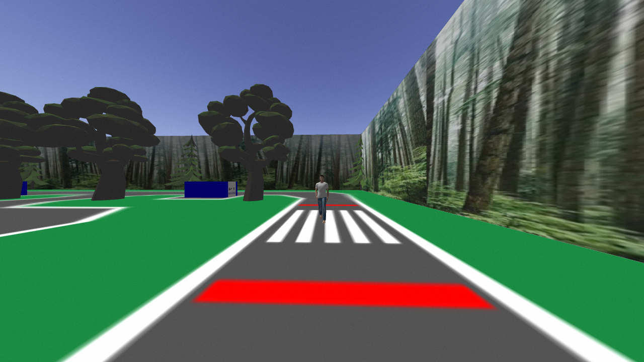
For detecting the crosswalk, pedestrian, and moving car, we masked specific colours that were attributed to those objects to detect when they are in frame. Specifically for license plate detection, we developed an image extraction algorithm which allows us to capture the license plates image from our robot, and feed it into a convolutional neural network which makes a prediction on what the letters and numbers are.
PID Controller and Object Detection
We implemented a PID controller for line following which drives our car around the track. We have set it up such that we can follow the lane based off of the left line or right line. This is useful because as we transition into our INNER state (corresponds to when we are driving in the inner ring), our controller takes the error off of the left line to turn left into the inner ring. To detect the white lines we take a small chunk of the camera frame of our robot, change to grayscale, and threshold it so we only see white lines. We average the columns of the matrix in order to capture the line geometry. A straight line would have values of the averaged array larger than if we were at the corner and the white line spanned across the horizontal more. We then set another threshold to determine the “centre” position of the white line which is what we take the error calculation based off of. This resulted with a well-balanced PID that is sensitive enough to follow a 90 degree bend while minimizing its oscillations.
Our strategy also requires us to detect the pedestrian, moving vehicle, crosswalk and cars. To do so, we convert the image into a hsv in order to mask specific colors (red for crosswalk, and blue for the pants of the pedestrian). To detect the moving vehicle, we just detect black color in the image by thresholding very low values. Lastly, we detect the black header of each car which allows us to count how many cars we passed. This is important in order to determine which parking number we are at.
Image Extraction Algorithm
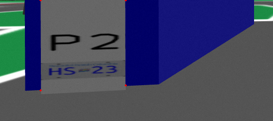
The goal for our image extraction algorithm was to quickly and consistently extract parking numbers and license plates. Several techniques were attempted before we settled on our chosen algorithm. Our first tests involved using SIFT to match a template license plate to the ones on the car directly from the simulation image. This proved ineffective since the detail from the simulation images was so blurred that SIFT could not match enough key points to obtain a homography, which would be the indicator of a “good match”. In the end we settled on a similar strategy to the gray masks but with the blue colour from the cars. This provided a clear indicator of the location of the rear of the car, and an image requiring less cleaning since there were no objects which were not a car that were blue.
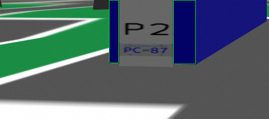
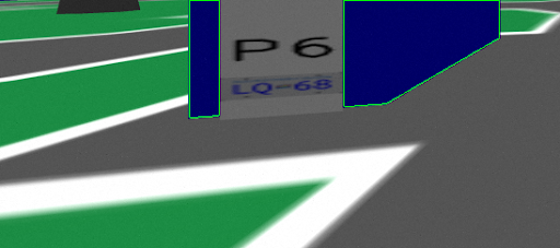
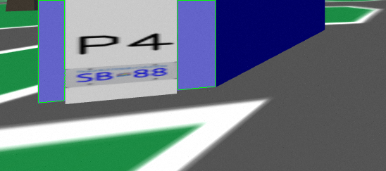
Image Preprocessing
We then used the OpenCV library’s findContours function to get a list of lists of points with each list corresponding to a shape in the image. For each shape in the image, we then calculated the maximum and minimum X and Y values from the points in the image, giving us a rectangle around the shape. We then chose the tallest rectangle from each colour mask; If it was shorter than a certain threshold value we would consider the image too small to contain a good image of the plate so the extraction operation would be halted.
If we found a shape with a similar height to the tallest one, which was tall enough to contain a good image, then we assumed it enclosed a license plate. Then once we had these two shapes we would compare their X values and arrange them horizontally. The points for the corners of the plate were then chosen by taking the maximum X values for the leftmost image and minimum X values for the rightmost image as the edges of the rear end of the car and then using the maximum and minimum Y of each shape to get the corner points. Once these points were selected, the image underwent a perspective transform using the OpenCV function getPerspectiveTransform which would result in a head on image of the rear of the car.
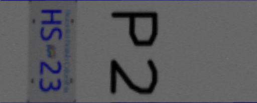
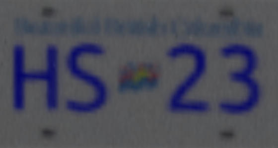
From the transformed image, we still had to extract the final license plate. We took advantage of the darker gray on the license itself compared to the rest of the image. After graysacling the image, we scanned the image for differences in intensity to determine the outline of the final plate. After cropping to the final plate, we had to crop to individual characters to publish onto a ROS topic which directs to our CNN.
Convolutional Neural Networks

Image Construction
We created images using a license generator script which creates similar images to the ones seen in the simulation. The structure of the resulting images contain a parking number (P1) on top, and the license plate on the bottom. Having this allowed us to generate specific images and numbers we wanted to train on more in case our model had any issues with those predictions.
Image Pre-processing
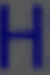
After we created some licenses, we had to crop the pictures like how we do in our image extraction pipeline. We do this because we chose our model to predict letters one at a time with high accuracy. After cropping, we apply gaussian blur to each of these images and save them to our local machines.
Image Transformation
After we crop our individual images, we used the ImageDataGenerator class from Keras which allows us to apply various transformations to the images. This allowed us to create more data that represents what we would actually see from our robot. Using this we were able to apply horizontal and vertical translation, rotation, zoom, brightness changes, and shear movement to all our images. This is our final step in creating images to train on. From all three of the steps above, we were able to create approximately 9000 images to train our model on which was the max that we could before our script crashes due to limited memory.
Model Development
We developed many different models that differ only in the amount of layers and kernel sizes. For example, we tried adding more Conv2D layers and changing their kernel size to see what affect it would have on the accuracy of our model. Other things we tried were changing our neural network layer and changing the amount of neurons in the deep layers. Ultimately we found that one of the largest impacts on our model was due to how we crop the images. We determine the shape of our crop from our image extraction pipeline, but because our generated images may be different size, the scale at which the number looks may be different in our generated images and the ones we actually see. Although we cropped the images to be of same size, we also resized them to make sure the scale size is the same as well. This helped our prediction immensely.
As our input shape is relatively smaller (150x100x3), we found that learning 32 filters in our conv2d layers was enough to capture important highlights of our data. We then reduced the representation with a maxpooling2d layer and then repeated this process twice. After, we flatten our data into one dimension, we then apply a dropout layer in order to reduce the complexity and prevent our model from overfitting. This will then feed into our first neural network layer of 128 nodes, then to a layer of 64 nodes, and then lastly 36 nodes which correspond to the 36 letters and numbers.
Training the Model
After developing our model, our final step is to train it. We obtain our labelled images from a file and create our X_dataset and Y_dataset. We normalize the data and shuffle so that our model does not overtrain. We split our training set and validation set 80% and 20% respectively. Our learning rate was 1e-4, and used a cross-entropy loss metric. This is often used for multi-class classification problems such as ours. We also used a RMSprop optimizer in order to change the weights and learning rate of our neural network automatically. This finalizes our entire training process!
